
Here are some examples of how to compute realistic Galactic orbits within NEMO. Again, as shown in the previous example, we first need to select a Galactic potential. To first order the motion in XY and Z are decoupled. We do have a very nice feature in NEMO, called potentials (and the newer 'accelerations' , not quite ready for release yet). Most programs use 3 keywords: potname=, potpars= and potfile= to use them, and have the same meaning for each program. potname identifies the type of potential (normally implemented in a file compiled as a shared object in $NEMOPOT/potential), potpars is used to add any (optional) real parameters to the potential, and potfile for any string based (e.g. filenames) parameters.
The Dehnen and Binney (1998, 1998MNRAS.294..429D) paper is exemplified in NEMO with a set of potentials in $NEMODAT/GalPot with the potname=GalPot potential descriptor. potfile= is used to point at the (ASCII) data file, and potpars is not used (except for pattern speeds, for which an example is also given below).
The units in GalPot potentials are kpc and km/s. First an example of how one creates an orbit. The LSR is usually defined (see also e.g. fig 10.9 in Binney & Merrifield, pp. 624) at position (-R0,0,0) and velocities (0,V0,0), i.e. the sun is rotating clockwise:

%  mkorbit orb1 x=-8.5 y=0 z=0 vx=0 vy=220 vz=0 potname=GalPot potfile=$NEMODAT/GalPot/pot.1
Using pattern speed = 0
pos: -8.500000 0.000000 0.000000
vel: 0.000000 220.000000 0.000000
etot: -129415.311558
lz=-1870.000000
The orbit is stored is stored in the file orb1, in an otherwise incomprehensible binary format, but the program tsf can be used to look at its contents in a slightly more human readable way:
%  tsf orb1
char History[122] "mkorbit orb1 x=-8.5 y=0 z=0 vx=0 vy=220 vz=0 potname
  =GalPot potfile=/astromake/opt/nemo/cvs/data/GalPot/pot.1 VERSION=4.0
  "
set Orbit
  set Parameters
    int Ndim 3
    double Mass 1.00000
    double IOM[3] -129415. -1870.00 0.00000
    double IOM_error[3] 0.00000 0.00000 0.00000
    int Nsteps 1
  tes
  set Potential
    char Name[7] "GalPot"
    char File[42] "/astromake/opt/nemo/cvs/data/GalPot/pot.1"
  tes
  set Path
    double TimePath[1] 0.00000
    double PhasePath[1][2][3] -8.50000 0.00000 0.00000 0.00000 220.000
      0.00000
  tes
tes

	==> BAD BUG: the $NEMODAT was expanded in my case, so this
	data isn't very portable!!!!
Now we need to integrate it. e.g.
orbint . With km/s and kpc
we have a timeunit of kpc/(km/s) of 1e9 yr (see also the command
units)
We "know" at 8.5 kpc and 220 km/s the orbital time is
2.pi.R/V, in NEMO I would be lazy and do
%  nemoinp '2*pi*8.5/220'
0.242759
i.e. 0.24 Gyr, or 240 Myr. Looks reasonable. I'm just doing a consistency check her, since I never even believe my own man pages or results. So, this means we can use integration steps of about 1/100 of this, so 0.2/100 = 0.002 or so. With 1000 steps that would be 10 orbits. Lets see how this looks, also storing EVERY integration step
%  orbint help=
orbint in=??? out=??? nsteps=10 dt=0.1 ndiag=0 nsave=1 potname= potpars=
potfile= mode=rk4 eta= variable=f VERSION=4.0a
gives a quick reminder to the keywords. Or if you like a little more detail on the keywords:
%  orbint help=h
in               : input filename (an orbit)  [???]
out              : output filename (an orbit)  [???]
nsteps           : number of steps [10]
dt               : (initial) timestep [0.1]
ndiag            : frequency of diagnostics output (0=none) [0]
nsave            : frequency of storing  [1]
potname          : potential name (default from orbit) []
potpars          : parameters of potential  []
potfile          : extra data-file for potential  []
mode             : integration method (euler,leapfrog,rk2,rk4) [rk4]
eta              : if used, stop if abs(de/e) > eta []
variable         : Use variable timesteps (needs eta=) [f]
VERSION          : 15-mar-04 PJT [4.0a]
Now we're ready to integrate. I'm cheating with the first few keywords, since i leave off the keyword= part, again for being lazy (if you write shell scripts, you should never do that since the order COULD change over the long term):
%  orbint orb1 orb1.out 1000 0.002 ndiag=100 nsave=1
 Pattern speed=0
0.000000 24200.000000 -153615.311558      -129415.3115583 -0
0.200000 25293.075518 -154708.388849      -129415.3133311 1.36988e-08
0.402000 27140.512276 -156555.827322      -129415.3150462 2.69512e-08
0.604000 26612.439215 -156027.756505      -129415.3172899 4.42884e-08
0.806000 24644.840425 -154060.160076      -129415.3196502 6.25268e-08
1.008000 24435.416517 -153850.738138      -129415.3216212 7.7757e-08
1.210000 26295.050958 -155710.374265      -129415.3233075 9.07867e-08
1.412000 27262.819891 -156678.145119       -129415.325228 1.05627e-07
1.614000 25634.041799 -155049.369439      -129415.3276395 1.24261e-07
1.816000 24216.004000 -153631.333827      -129415.3298264 1.41159e-07
Energy conservation: 1.41159e-07
that's pretty good energy conservation.
Now up to some plotting:
%  orbplot orb1.out xrange=-16:16 yrange=-16:16
Read orbit with 1001 phase-points
should bring up a PGPLOT screen if you installed it with pgplot (the default for most who use nemo) that should look something like the following plot:
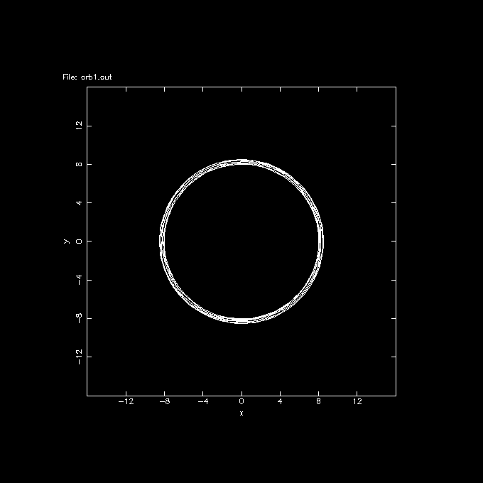
well, this is an example i got, hope you'll get the same, in which case you're on the way. most of the magic will be in selecting the potfile (or potname) and potpars, and initial conditions. If you want to play with a more statistical approach, i would use potcode, which can integrate it like an Nbody system (but as test particles). This way we can plot lindblad diagrams, and other kinds of plots to better compare with observations.
Note the orbit isn't exactly circular, I was sloppy in providing old style 220 km/s @ 8.5 kpc for the LSR, not appropriate for this particular model. We leave it as an excersize for the reader to find the exact circular orbit.
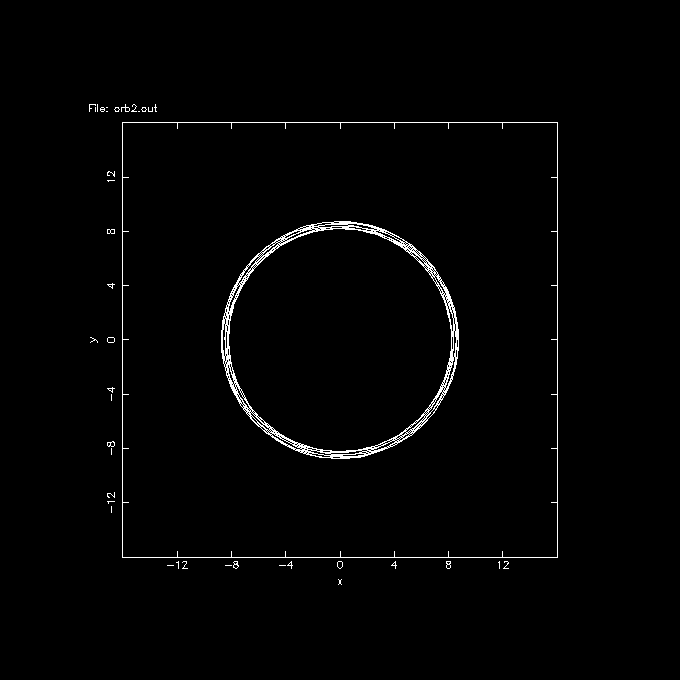
To calculate the orbit of the sun, compared to the LSR, we take the UVW components of (10.0,5.2.7.2) and observe:
%  mkorbit orb2 x=-8.5 y=0 z=0 vx=10.0 vy=220+5.2 vz=7.2 potname=GalPot potfile=$NEMODAT/GalPot/pot.1
Using pattern speed = 0
pos: -8.500000 0.000000 0.000000
vel: 10.000000 225.200000 7.200000
etot: -128181.871558
lz=-1914.200000

                               Note one can use most common math operations on the commandline, such at 220+5.2

%  orbint orb2 orb2.out 1000 0.002 ndiag=100 nsave=1
Pattern speed=0
0.000000 25433.440000 -153615.311558      -128181.8715583 5.67628e-17
0.200000 27042.342182 -155224.216839      -128181.8746572 2.41758e-08
0.402000 27063.028724 -155244.905440      -128181.8767154 4.02329e-08
0.604000 25285.944917 -153467.834640      -128181.8897234 1.41713e-07
0.806000 24061.614228 -152243.506322      -128181.8920934 1.60203e-07
1.008000 24693.346633 -152875.241959      -128181.8953256 1.85418e-07
1.210000 26542.966561 -154724.868257      -128181.9016969 2.35123e-07
1.412000 27322.213854 -155504.110917      -128181.8970627 1.98971e-07
1.614000 25975.220080 -154157.120744      -128181.9006632 2.2706e-07
1.816000 24299.104184 -152480.998253       -128181.894069 1.75615e-07
Energy conservation: 1.75615e-07

%  orbplot orb2.out xrange=-16:16 yrange=-16:16 yapp=GalPot2.gif/gif
It would be more interesting to view the orbit in the rotating frame of reference. For this we first need to compute the pattern speed at an assumed LSR. We can use rotcurves for this. Although this program can compute and plot a whole rotation curve, we're only interested in the R=8.5 point:
%  rotcurves GalPot 0 $NEMODAT/GalPot/pot.1 radii=8.5 tab=t yapp=/null
Pattern speed: 0.000000
8.500000 226.483488

%  nemoinp  226.483488/8.5
26.6451
                note the solar orbit is clock-wise, which is a negative pattern speed

%  mkorbit orb3 x=-8.5 y=0 z=0 vx=10.0 vy=5.2 vz=7.2 potname=GalPot potfile=$NEMODAT/GalPot/pot.1 potpars=-26.6451
Using pattern speed = -26.6451
pos: -8.500000 0.000000 0.000000
vel: 10.000000 5.200000 7.200000
etot: -179173.225472
lz=-44.200000

                no need to re-specify potential parameters, the defaults are now inside the datafile

%  orbint orb3 orb3.out 1000 0.002 ndiag=100 nsave=1
Pattern speed=-26.6451
0.000000 89.440000 -179262.665472      -179173.2254719 1.30074e-17
0.200000 96.247953 -179269.473359      -179173.2254059 -3.68405e-10
0.402000 77.178398 -179250.404005      -179173.2256069 7.53669e-10
0.604000 148.951337 -179322.179418      -179173.2280807 1.456e-08
0.806000 288.141667 -179461.372681      -179173.2310136 3.09292e-08
1.008000 271.385295 -179444.615048      -179173.2297529 2.38932e-08
1.210000 132.094065 -179305.327056      -179173.2329912 4.19666e-08
1.412000 88.329109 -179261.556716      -179173.2276071 1.19172e-08
1.614000 100.854240 -179274.083465      -179173.2292249 2.09463e-08
1.816000 90.661651 -179263.892740      -179173.2310885 3.13471e-08
Energy conservation: 3.13471e-08

%  orbplot orb3.out xrange=-16:16 yrange=-16:16
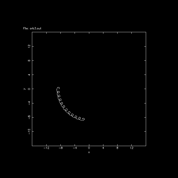
This shows the orbit of the sun is trailing the LSR, in fact in 2Gyr it looks like almost 1/4 of an orbit! Although that's an interesting plot, you can also see the epicyclic frequency is a lot higher than the angular. In 1/4 turn it has executed almost 10 epicycles!
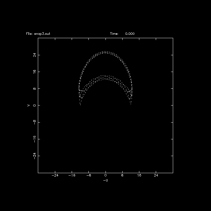
The last thing to show in this demo are the UVW coordinates. These are the velocities in the radial, angular in the direction of solar motion, and vertical direction, all relative to the LSR. Unfortunately, the orbit routines in NEMO do not have as sophisticated analysis options as the ones that handle snapshots, yet they contain the same data. Thus it is easier (for now) to convert the orbit using otos to a set of snapshots (like a long series of integrated 1-body models), and use snapplot to plot the -U and V coordinates:
%  otos orb3.out snap3.out

%  snapplot snap3.out xrange=-32:32 yrange=-32:32 xvar=vr yvar=vt xlabel=-U ylabel=V
  unfinished examples:
  show blowup of current solar orbit:

  integrate in reverse:

   orbint orb3 orb3r.out 1000 -0.002 ndiag=100 nsave=1

  paste and plot, also showing a bit more use of pipes in NEMO

   cat orb3.out orb3r.out | orbplot - xrange=-11:-7 yrange=-2:2

  this should show
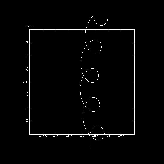
A more sophisticated shell script version of the above can be found here. You will find that some of the models produce interesting looking asymmetric shapes in the UV projection, e.g. n=4e.
This page was last modified on by PJT.