The program eaglesnap is an alternative to the otherwise much nicer python interfaces of martini to make mock observations of EAGLE simulations. Nonetheless we will show here a few of the things one can do with NEMO. Keep in mind that in the current version units are still code-units, and the time is always fixed at 0.0.
If you want to play with this yourself, you will need to get an account to download the EAGLE data, so the remainder of this page assumes you have done that.
  wget --user=??? --ask-password --content-disposition
      "http://dataweb.cosma.dur.ac.uk:8080/eagle-snapshots//download?run=RefL0012N0188&snapnum=28"
  wget --user=??? --ask-password --content-disposition
      "http://dataweb.cosma.dur.ac.uk:8080/eagle-snapshots//download?run=RefL0012N0188&snapnum=0"
  tar xvf RefL0012N0188_snap_028.tar
  tar xvf RefL0012N0188_snap_000.tar

  h5dump RefL0012N0188/snapshot_028_z000p000/snap_028_z000p000.0.hdf5 | more

  eaglesnap RefL0012N0188/snapshot_028_z000p000/snap_028_z000p000.0.hdf5 snap1  ptype=0 region=2
  ### nemo Debug Info: Region: 0,2 0,2 0,2
  ### nemo Debug Info: Found 97418 particles of type 0
  ### nemo Debug Info: GroupNumber: 82 - 4064
  ### nemo Debug Info: Writing 97418 particles (group -1, subgroup -1)


  tsf snap1
  char History[106] "eaglesnap RefL0012N0188/snapshot_028_z000p000/snap_028_z000p000.0.hdf5 snap1 ptype=0 region=2 VERSION=0.5"
  set SnapShot
    set Parameters
      int Nobj 97418
      double Time 0.00000
    tes
    set Particles
      int CoordSystem 66306
      double Mass[97418] 0.000122525 0.000122525 0.000122525 0.000122525 0.000122525 0.000122525 0.000122525 0.000122525 0.000122525
        0.000122525 0.000122525 0.000122525 0.000122525 0.000122525 0.000122525 0.000122525 0.000122525 0.000122525 0.000122525 0.000122525
        0.000122525 0.000122525 0.000122525 0.000122525 0.000122525 0.000122525 0.000122525 0.000122525 0.000122735 0.000122525 0.000122525
        0.000122525 0.000122525 0.000122525 0.000122525 0.000122525 0.000122525 0.000122525 0.000122525 0.000122525 0.000122525 0.000122525
        . . .
      double PhaseSpace[97418][2][3] 0.105699 0.110451 0.0599183 48.6903 47.3848 -11.4336 0.105796 0.0433156 0.00545288 36.9015 40.5002
        -14.4235 0.0731210 0.0403979 0.0853803 15.6860 39.7792 -7.38430 0.127888 0.113369 0.128862 30.6164 64.7130 -3.80271 0.0281841 0.112213
        0.232397 7.04478 71.5050 7.75067 0.103734 0.0971262 0.228682 14.7581 74.5385 -6.10375 0.129609 0.0309282 0.208724 -0.576880 70.5228
        -12.0157 0.228777 0.0722076 0.147447 19.3806 67.5598 4.41063 0.210431 0.0381443 0.235125 2.01781 62.2223 -12.8504 0.209561 0.0204466
        . . .
    tes
  tes
The ptype=0 refers to the gas, the region=0 will extract a small cube
from 0 to 2 in both X,Y and Z. Only 97418 particles are
extracted. Also note that version 0.5 of eaglesnap was used to extract
this data, with all of its (units) shortcomings.
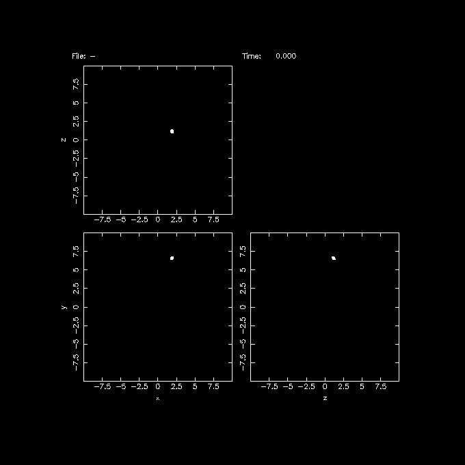
  eaglesnap RefL0012N0188/snapshot_028_z000p000/snap_028_z000p000.0.hdf5 - 0 group=2 |\
  snapplot3 - xrange=-10:10 yrange=-10:10 zrange=-10:10
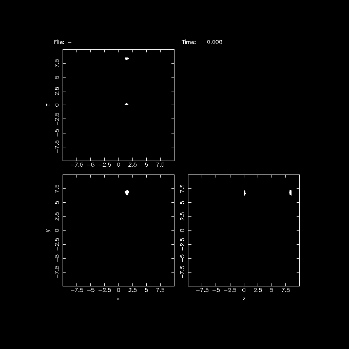
  eaglesnap RefL0012N0188/snapshot_028_z000p000/snap_028_z000p000.0.hdf5 - 0 group=4 |\
  snapplot3 - xrange=-10:10 yrange=-10:10 zrange=-10:10
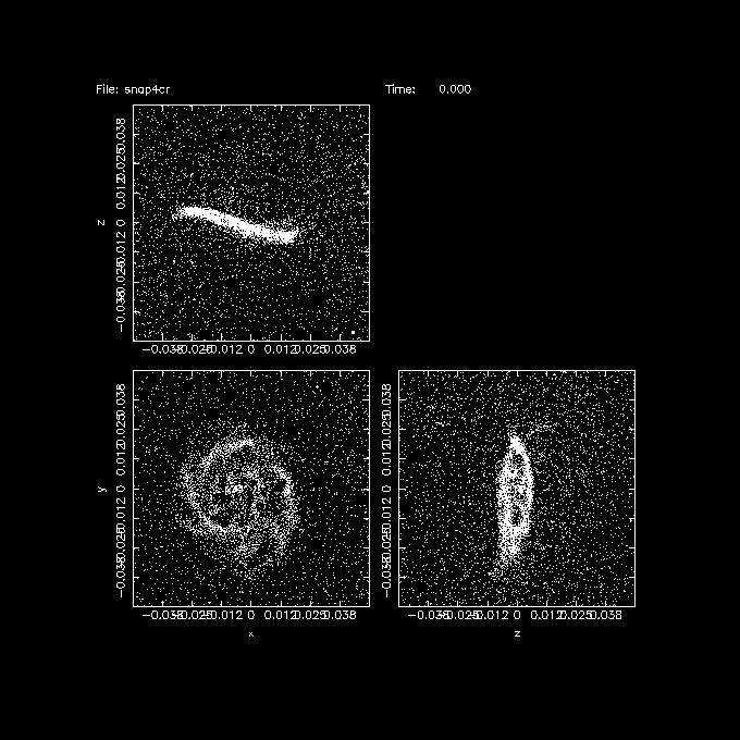
  eaglesnap snap_028_z000p000.0.hdf5 - 0 group=4 center=1.9,6.6,1.2 boxsize=8.47125 |\
  hackforce - - |\
  snapcenter - - '-phi*phi*phi' |\
  snaprect - snap4cr '-phi*phi*phi'

  s=0.05
  snapplot3 snap4cr xrange=-$s:$s yrange=-$s:$s zrange=-$s:$s
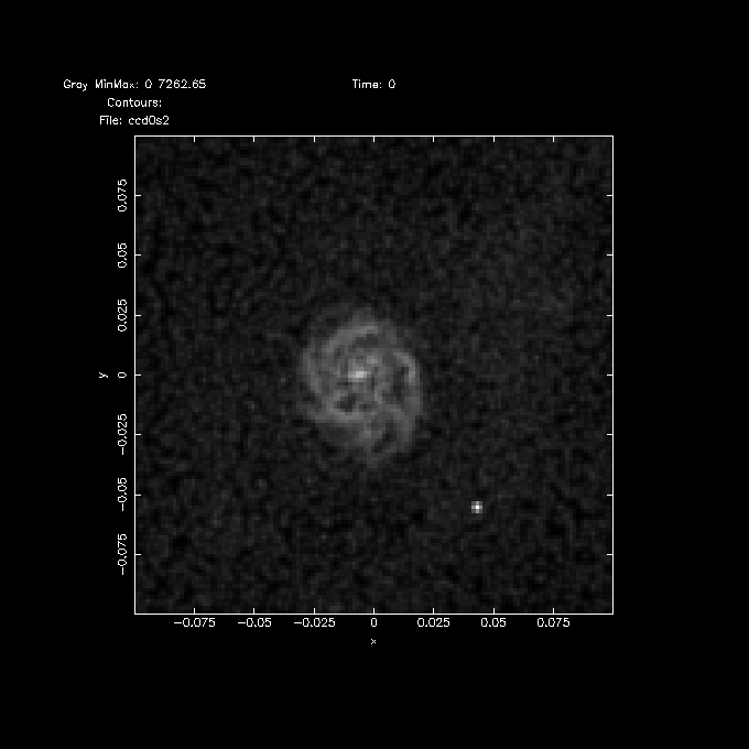
  s=0.1
  snapgrid snap4cr ccd0s xrange=-$s:$s yrange=-$s:$s nx=128 ny=128 mom=0  svar=0.001
  snapgrid snap4cr ccd1s xrange=-$s:$s yrange=-$s:$s nx=128 ny=128 mom=-1 svar=0.001
  ccdplot ccd0s power=0.5
  ccdplot ccd1s
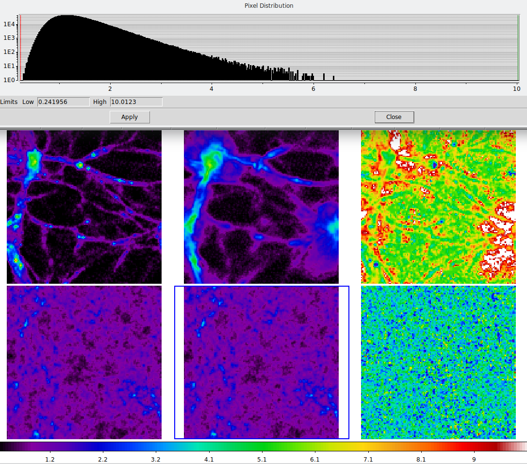
  b=8.47125      # box size
  dm=4365.77     # cheat to get the correct DM amount

  eaglesnap snapshot_028_z000p000/snap_028_z000p000.0.hdf5 - 0 |\
  snapgridsmooth - -  xrange=0:$b yrange=0:$b zrange=0:$b nx=128 ny=128 nz=128 periodic=t |\
  ccdsmooth - gas0s 0.1 dir=xyz

  eaglesnap snapshot_028_z000p000/snap_028_z000p000.0.hdf5 - 1 dm=$dm |\
  snapgridsmooth - -  xrange=0:$b yrange=0:$b zrange=0:$b nx=128 ny=128 nz=128 periodic=t |\
  ccdsmooth - dm0s 0.1 dir=xyz

  eaglesnap snapshot_000_z020p000/snap_000_z020p000.0.hdf5 - 0 |\
  snapgridsmooth - -  xrange=0:$b yrange=0:$b zrange=0:$b nx=128 ny=128 nz=128 periodic=t |\
  ccdsmooth - gas20s 0.1 dir=xyz

  eaglesnap snapshot_000_z020p000/snap_000_z020p000.0.hdf5 - 1 dm=$dm |\
  snapgridsmooth - -  xrange=0:$b yrange=0:$b zrange=0:$b nx=128 ny=128 nz=128 periodic=t |\
  ccdsmooth - dm20s 0.1 dir=xyz

  # compute masses
  ccdstat gas0s
  -> Sum and Sum*Dx*Dy*Dz*  : 2706454.922333 784.536918
  ccdstat dm0s
  -> Sum and Sum*Dx*Dy*Dz*  : 14849409.591463 4304.490697
  ccdstat gas20s
  -> Min and Max            : 0.241956 10.012325
  -> Mean and dispersion    : 1.327166 0.430398
  -> Sum and Sum*Dx*Dy*Dz*  : 2783269.386730 806.803604
  ccdstat dm20s
  -> Min and Max            : 1.507509 54.906773
  -> Mean and dispersion    : 7.116934 2.306722
  -> Sum and Sum*Dx*Dy*Dz*  : 14925292.575197 4326.487370

  # compute local Baryonic Fraction
  ccdmath gas20s,dm20s bf20 %1/%2
  ccdmath gas0s,dm0s   bf0  %1/%2

  ccdstat bf20
  -> Min and Max            : 0.092280 0.339595
  -> Mean and dispersion    : 0.187254 0.017474

  ccdstat bf0
  -> Min and Max            : 0.000000 10459.553627
  -> Mean and dispersion    : 0.937404 13.933238
  cd $NEMO/usr/eagle
  make install
  mknemo eaglesnap
but it may also require some other tweaking. Version 4.2 of NEMO should fully resolve this.
This page was last modified on by PJT.